Search Finite Elements Website

Strain

 home > basic mechanics > strain

Introduction

This page presents the so-called infinitesimal strains, though it is a bit of a misnomer because it is actually rotations that need to be small, not the strains themselves, in order to accurately use the small strain equations. For those interested, a complete discussion of the limitations of infinitesimal strain definitions can be found here: http://www.continuummechanics.org/smallstrain.html.

---

Normal Strains

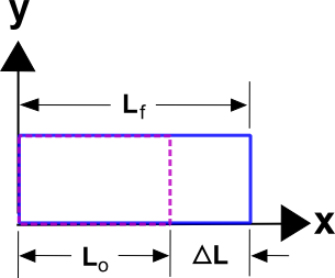
Normal in normal strain does not mean common, or usual strain. It means a direct length-changing stretch (or compression) of an object resulting from a normal stress. It is commonly defined as

\[ \epsilon = {\Delta L \over L_o} \]
where the quantities are defined in the sketch. This is also known as Engineering Strain. Note that when \(\Delta L\) is small, then \(L_o\) will be so close to \(L_f\) that the specification of either in the denominator of \(\Delta L / L\) is unnecessary, in fact. This will be assumed to be the case throughout this page.

The definition arises from the fact that if a 1 m long rope is pulled and fails after it stretches 0.015 m, then we would expect a 10 m rope to stretch 0.15 m before it fails. In each case, the strain is \(\epsilon\) = 0.015, or 1.5%, and is a constant value independent of the rope's length, even though the \(\Delta L's\) are different values in the two cases. Likewise, the force required to stretch a rope by a given amount would be found to depend only on the strain in the rope. It is this foundational concept of strain that makes this definition a useful choice.

---

Shear Strains

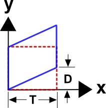
Shear strain is usually represented by \(\gamma\) and defined as

\[ \gamma = {D \over T} \]
This is the shear-version of engineering strain. Note that this situation does include some rigid body rotation because the square tends to rotate counter-clockwise here, but we will ignore this complication for now.

---

---

Pure Shear Strains

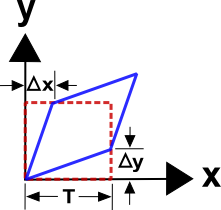
So a better, but slightly more complex definition of shear strain, is

\[ \gamma = { \Delta x + \Delta y \over T} \]
where it is assumed that the starting point is also a square. It should be noted that the two definitions lead to the same results when the displacements and strains are small. In other words

\[ \Delta x = \Delta y = { D \over 2} \qquad \text{(small strains)} \]
This permits one to think in terms of the first definition while using the second.

---

General Definitions

The above definitions are good in that they work for simple cases in which all the strain is one or the other (normal or shear). But as soon as the strain components are simultaneously present for \(\epsilon_x, \epsilon_y, \epsilon_z, \gamma_{xy}\), etc., things can become unmanageable. So a more general method of calculation is needed.

The answer to this dilemma is... calculus. The approach is to define the various strains in terms of partial derivatives of the displacement field, \({\bf u({\bf X})}\), in such a way that the above definitions are preserved for the simple cases.

Normal Strains

The normal strains are defined as

\[ \epsilon_x = {\partial \, u_x \over \partial X} \qquad \epsilon_y = {\partial \, u_y \over \partial Y} \qquad \epsilon_z = {\partial \, u_z \over \partial Z} \]
The simple case of uniaxial stretching can be described as

\[ x = \left( {X \over L_o} \right) L_f \]
and since \({\bf u} = {\bf x} - {\bf X}\), a little algebra can be applied to give

\[ u_x = \left( {X \over L_o} \right) \left( L_f - L_o \right) \]
So

\[ \epsilon_x \quad = \quad {\partial \, u_x \over \partial X} \quad = \quad {L_f - L_o \over L_o} \quad = \quad {\Delta L \over L_o} \]
which reproduces the "delta L over L" definition as desired.

Shear Strains

The equation for shear strain is


\[ \gamma_{xy} = {\partial \, u_y \over \partial X} + {\partial \, u_x \over \partial Y} \]
The coordinate mapping equation for the shear example is

\[ \begin{eqnarray} x & = & X \\ y & = & Y + X D / T \end{eqnarray} \]
And the displacement field is

\[ \begin{eqnarray} u_x & = & 0 \\ u_y & = & X D / T \end{eqnarray} \]
The shear strain is

\[ \gamma_{xy} \quad = \quad {\partial \, u_y \over \partial X} + {\partial \, u_x \over \partial Y} \quad = \quad {\partial \, (X D / T) \over \partial X} + {\partial \, (0) \over \partial Y} \quad = \quad {D \over T} \]
This reproduces the desired result for this simple case: \(\gamma_{xy} = D / T\).

The symmetry of the equation also ensures that the computed shear value also satisfies the no-net-rotation criterion. The coordinate mapping equations for this example are


\[ \begin{eqnarray} x & = & X & + & Y \Delta x / T \\ y & = & Y & + & X \Delta y / T \end{eqnarray} \]
and they lead to

\[ \gamma_{xy} = {\Delta x + \Delta y \over T} \]
which again produces the desired result.

---

2-D Notation

Strain, like stress, is a tensor. And like stress, strain is a tensor simply because it obeys the standard coordinate transformation principles of tensors. It can be written in any of several different forms as follows. They are all identical.

\[ \boldsymbol{\epsilon} = \left[ \matrix{ \epsilon_{11} & \epsilon_{12} \\ \epsilon_{21} & \epsilon_{22} } \right] = \left[ \matrix{ \epsilon_{xx} & \epsilon_{xy} \\ \epsilon_{yx} & \epsilon_{yy} } \right] = \left[ \matrix{ \epsilon_{xx} & \gamma_{xy}/2 \\ \gamma_{yx}/2 & \epsilon_{yy} } \right] \]
But since \(\gamma_{xy} = \gamma_{yx}\), all the tensors can also be written as

\[ \boldsymbol{\epsilon} = \left[ \matrix{ \epsilon_{11} & \epsilon_{12} \\ \epsilon_{12} & \epsilon_{22} } \right] = \left[ \matrix{ \epsilon_{xx} & \epsilon_{xy} \\ \epsilon_{xy} & \epsilon_{yy} } \right] = \left[ \matrix{ \epsilon_{xx} & \gamma_{xy}/2 \\ \gamma_{xy}/2 & \epsilon_{yy} } \right] \]
Setting \(\gamma_{xy} = \gamma_{yx}\) has the effect of making (requiring in fact) the strain tensors symmetric.

---

3-D Notation

All of the above conventions in 2-D also apply to the 3-D case. Notation for the 3-D case is as follows.

\[ \boldsymbol{\epsilon} = \left[ \matrix{ \epsilon_{11} & \epsilon_{12} & \epsilon_{13} \\ \epsilon_{21} & \epsilon_{22} & \epsilon_{23} \\ \epsilon_{31} & \epsilon_{32} & \epsilon_{33} } \right] = \left[ \matrix{ \epsilon_{xx} & \epsilon_{xy} & \epsilon_{xz} \\ \epsilon_{yx} & \epsilon_{yy} & \epsilon_{yz} \\ \epsilon_{zx} & \epsilon_{zy} & \epsilon_{zz} } \right] = \left[ \matrix{ \epsilon_{xx} & \gamma_{xy}/2 & \gamma_{xz}/2 \\ \gamma_{yx}/2 & \epsilon_{yy} & \gamma_{yz}/2 \\ \gamma_{zx}/2 & \gamma_{zy}/2 & \epsilon_{zz} } \right] \]
But rotational equilibrium requires that \(\gamma_{xy} = \gamma_{yx}\), \(\gamma_{xz} = \gamma_{zx}\), and \(\gamma_{yz} = \gamma_{zy}\). This also produces symmetric tensors.

\[ \boldsymbol{\epsilon} = \left[ \matrix{ \epsilon_{11} & \epsilon_{12} & \epsilon_{13} \\ \epsilon_{12} & \epsilon_{22} & \epsilon_{23} \\ \epsilon_{13} & \epsilon_{23} & \epsilon_{33} } \right] = \left[ \matrix{ \epsilon_{xx} & \epsilon_{xy} & \epsilon_{xz} \\ \epsilon_{xy} & \epsilon_{yy} & \epsilon_{yz} \\ \epsilon_{xz} & \epsilon_{yz} & \epsilon_{zz} } \right] = \left[ \matrix{ \epsilon_{xx} & \gamma_{xy}/2 & \gamma_{xz}/2 \\ \gamma_{xy}/2 & \epsilon_{yy} & \gamma_{yz}/2 \\ \gamma_{xz}/2 & \gamma_{yz}/2 & \epsilon_{zz} } \right] \]